TL;DR
本章的目标依然是学习一种模型 $\hat{y}$,能准确对输入 $X$ 及对应的输出 $y$ 进行建模。
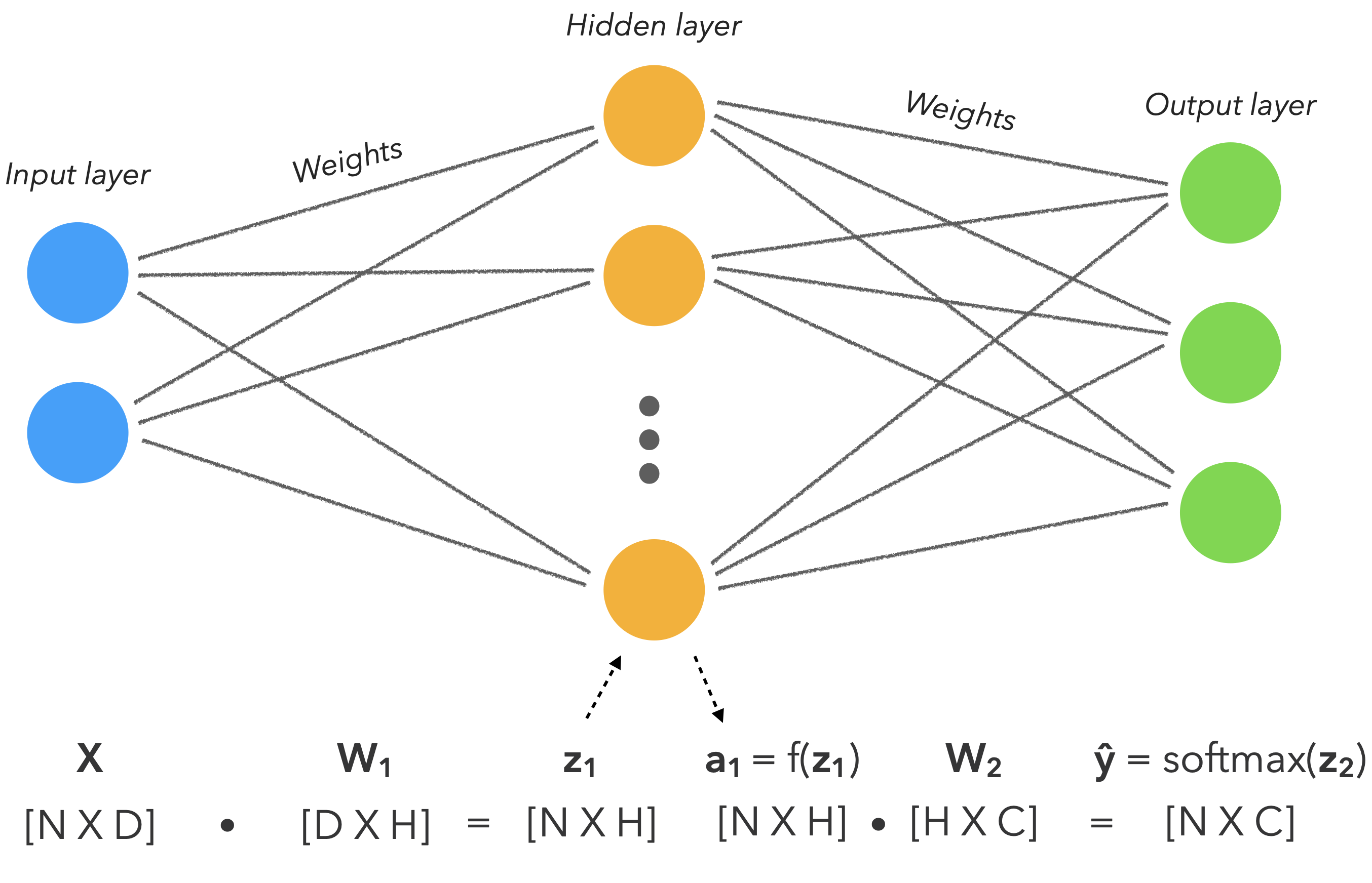
你会注意到神经网络只是我们迄今为止看到的广义线性方法的扩展,但具有非线性激活函数,因为我们的数据是高度非线性的。
$$
$$
$$
$$
参数
解释
$N$
样本数
$D$
特征数
$H$
隐藏神经元
$C$
标签数
$W_1$
第一层的权重
$z_1$
第一层的输出
$f$
非线性激活函数
$a_1$
第一层的激活值
$W_2$
第二层的权重
$z_2$
第二层的输出
Set up
1
2
3
4
5
6
7
8
import numpy as npimport randomSEED = 1024 np.random.seed(SEED) random.seed(SEED)
Load data
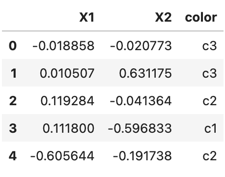
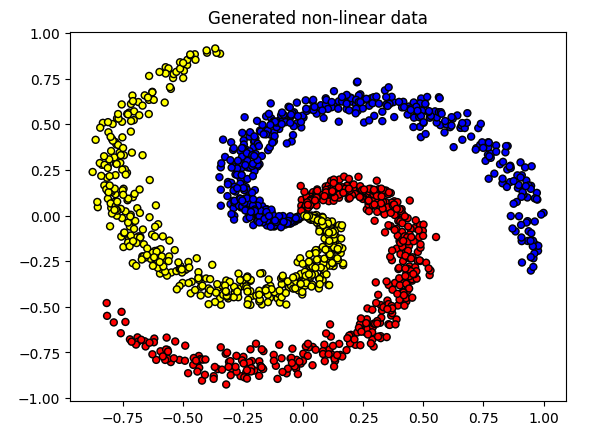
这里准备了一份非线性可分的螺旋数据来学习。
1
2
3
4
5
6
7
8
import matplotlib.pyplot as pltimport pandas as pdurl = "http://s3.mindex.xyz/datasets/9378f64fc8dd2817e4c92be0a3bae8e7.csv" df = pd.read_csv(url, header=0 ) df = df.sample(frac=1 ).reset_index(drop=True ) df.head()
1 2 3 4 5 6 7 8 9 10 11 12 13 14 15 X = df[["X1" , "X2" ]].values y = df["color" ].values print ("X: " , np.shape(X))print ("y: " , np.shape(y))plt.title("Generated non-linear data" ) colors = {"c1" : "red" , "c2" : "yellow" , "c3" : "blue" } plt.scatter(X[:, 0 ], X[:, 1 ], c=[colors[_y] for _y in y], edgecolors="k" , s=25 ) plt.show()
Split data
1
2
3
4
5
6
7
8
9
10
11
12
13
14
15
16
17
18
19
20
21
22
23
24
25
import collectionsfrom sklearn.model_selection import train_test_splitTRAIN_SIZE = 0.7 VAL_SIZE = 0.15 TEST_SIZE = 0.15 def train_val_test_split (X, y, train_size ): X_train, X_, y_train, y_ = train_test_split(X, y, train_size=TRAIN_SIZE, stratify=y) X_test, X_val, y_test, y_val = train_test_split(X_, y_, train_size=0.5 , stratify=y_) return X_train, X_val, X_test, y_train, y_val, y_test X_train, X_val, X_test, y_train, y_val, y_test = train_val_test_split( X=X, y=y, train_size=TRAIN_SIZE) print (f"X_train: {X_train.shape} , y_train: {y_train.shape} " )print (f"X_val: {X_val.shape} , y_val: {y_val.shape} " )print (f"X_test: {X_test.shape} , y_test: {y_test.shape} " )print (f"Sample point: {X_train[0 ]} → {y_train[0 ]} " )
Label encoding
1
2
3
4
5
6
7
8
9
10
11
12
13
14
15
16
17
18
19
20
21
22
23
24
25
26
27
28
29
30
31
32
33
34
from sklearn.preprocessing import LabelEncoderlabel_encoder = LabelEncoder() label_encoder = label_encoder.fit(y_train) classes = list (label_encoder.classes_) print (f"classes: {classes} " )print (f"y_train[0]: {y_train[0 ]} " )y_train = label_encoder.transform(y_train) y_val = label_encoder.transform(y_val) y_test = label_encoder.transform(y_test) print (f"y_train[0]: {y_train[0 ]} " )counts = np.bincount(y_train) class_weights = {i: 1.0 /count for i, count in enumerate (counts)} print (f"counts: {counts} \nweights: {class_weights} " )
Standardize data
因为 $y$ 是类别值,所以我们只标准化 $X$
1
2
3
4
5
6
7
8
9
10
11
12
13
14
15
16
17
from sklearn.preprocessing import StandardScalerX_scaler = StandardScaler().fit(X_train) X_train = X_scaler.transform(X_train) X_val = X_scaler.transform(X_val) X_test = X_scaler.transform(X_test) print (f"X_test[0]: mean: {np.mean(X_test[:, 0 ], axis=0 ):.1 f} , std: {np.std(X_test[:, 0 ], axis=0 ):.1 f} " )print (f"X_test[1]: mean: {np.mean(X_test[:, 1 ], axis=0 ):.1 f} , std: {np.std(X_test[:, 1 ], axis=0 ):.1 f} " )
Linear model
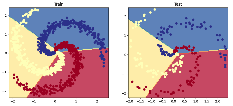
在尝试使用神经网络之前,为了解释激活函数,我们先用前面学到的逻辑回归模型来学习我们的数据。
你会发现一个用线性激活函数的线性模型对我们的数据来说并不是合适的。
Model & Train
1
2
3
4
5
6
7
8
9
10
11
12
13
14
15
16
17
18
19
20
21
22
23
24
25
26
27
28
29
30
31
32
33
34
35
36
37
38
39
40
41
42
43
44
45
46
47
48
49
50
51
52
53
54
55
56
57
58
59
60
61
62
63
64
65
66
67
68
69
70
71
72
73
74
75
76
77
78
79
80
81
82
83
84
import torchfrom torch import nnimport torch.nn.functional as Ffrom torch.optim import AdamINPUT_DIM = X_train.shape[1 ] HIDDEN_DIM = 100 NUM_CLASSES = len (classes) class LinearModel (nn.Module): def __init__ (self, input_dim, hidden_dim, num_classes ): super (LinearModel, self).__init__() self.fc1 = nn.Linear(input_dim, hidden_dim) self.fc2 = nn.Linear(hidden_dim, num_classes) def forward (self, x_in ): z = self.fc1(x_in) z = self.fc2(z) return z model = LinearModel(input_dim=INPUT_DIM, hidden_dim=HIDDEN_DIM, num_classes=NUM_CLASSES) LEARNING_RATE = 1e-2 NUM_EPOCHS = 10 BATCH_SIZE = 32 class_weights_tensor = torch.Tensor(list (class_weights.values())) loss_fn = nn.CrossEntropyLoss(weight=class_weights_tensor) def accuracy_fn (y_pred, y_true ): n_correct = torch.eq(y_pred, y_true).sum ().item() accuracy = (n_correct / len (y_pred)) * 100 return accuracy optimizer = Adam(model.parameters(), lr=LEARNING_RATE) X_train = torch.Tensor(X_train) y_train = torch.LongTensor(y_train) X_val = torch.Tensor(X_val) y_val = torch.LongTensor(y_val) X_test = torch.Tensor(X_test) y_test = torch.LongTensor(y_test) for epoch in range (NUM_EPOCHS): y_pred = model(X_train) loss = loss_fn(y_pred, y_train) optimizer.zero_grad() loss.backward() optimizer.step() if epoch%1 ==0 : predictions = y_pred.max (dim=1 )[1 ] accuracy = accuracy_fn(y_pred=predictions, y_true=y_train) print (f"Epoch: {epoch} | loss: {loss:.2 f} , accuracy: {accuracy:.1 f} " )
Evaluation
我们来看一下这个线性模型在螺旋数据上的表现如何。
1
2
3
4
5
6
7
8
9
10
11
12
13
14
15
16
17
18
19
20
21
22
23
24
25
26
27
28
29
30
31
32
33
34
35
36
37
38
39
40
41
42
43
44
45
46
47
48
49
50
51
52
53
54
55
56
57
58
59
60
61
62
63
64
65
66
67
68
69
70
71
72
73
74
75
76
77
78
79
80
81
82
83
84
85
86
87
88
89
90
91
92
93
94
95
96
97
98
import jsonimport matplotlib.pyplot as pltfrom sklearn.metrics import precision_recall_fscore_supportdef get_metrics (y_true, y_pred, classes ): """Per-class performance metrics.""" performance = {"overall" : {}, "class" : {}} metrics = precision_recall_fscore_support(y_true, y_pred, average="weighted" ) performance["overall" ]["precision" ] = metrics[0 ] performance["overall" ]["recall" ] = metrics[1 ] performance["overall" ]["f1" ] = metrics[2 ] performance["overall" ]["num_samples" ] = np.float64(len (y_true)) metrics = precision_recall_fscore_support(y_true, y_pred, average=None ) for i in range (len (classes)): performance["class" ][classes[i]] = { "precision" : metrics[0 ][i], "recall" : metrics[1 ][i], "f1" : metrics[2 ][i], "num_samples" : np.float64(metrics[3 ][i]), } return performance y_prob = F.softmax(model(X_test), dim=1 ) print (f"sample probability: {y_prob[0 ]} " )y_pred = y_prob.max (dim=1 )[1 ] print (f"sample class: {y_pred[0 ]} " )performance = get_metrics(y_true=y_test, y_pred=y_pred, classes=classes) print (json.dumps(performance, indent=2 ))def plot_multiclass_decision_boundary (model, X, y ): x_min, x_max = X[:, 0 ].min () - 0.1 , X[:, 0 ].max () + 0.1 y_min, y_max = X[:, 1 ].min () - 0.1 , X[:, 1 ].max () + 0.1 xx, yy = np.meshgrid(np.linspace(x_min, x_max, 101 ), np.linspace(y_min, y_max, 101 )) cmap = plt.cm.Spectral X_test = torch.from_numpy(np.c_[xx.ravel(), yy.ravel()]).float () y_pred = F.softmax(model(X_test), dim=1 ) _, y_pred = y_pred.max (dim=1 ) y_pred = y_pred.reshape(xx.shape) plt.contourf(xx, yy, y_pred, cmap=plt.cm.Spectral, alpha=0.8 ) plt.scatter(X[:, 0 ], X[:, 1 ], c=y, s=40 , cmap=plt.cm.RdYlBu) plt.xlim(xx.min (), xx.max ()) plt.ylim(yy.min (), yy.max ()) plt.figure(figsize=(12 ,5 )) plt.subplot(1 , 2 , 1 ) plt.title("Train" ) plot_multiclass_decision_boundary(model=model, X=X_train, y=y_train) plt.subplot(1 , 2 , 2 ) plt.title("Test" ) plot_multiclass_decision_boundary(model=model, X=X_test, y=y_test) plt.show()
Activation functions
使用广义的线性方法产生了较差的结果,因为我们试图用线性激活函数去学习非线性数据。
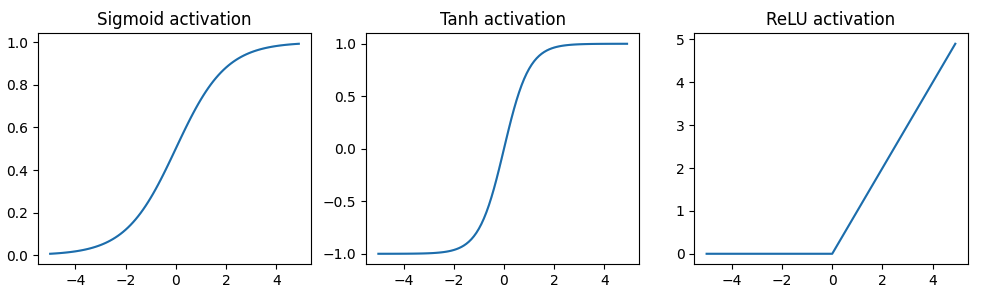
所以我们需要一个可以能让模型学习到数据中的非线性的激活函数。有几种不同的选择,我们稍微探索一下。
1 2 3 4 5 6 7 8 9 10 11 12 13 14 15 16 17 18 19 20 21 22 23 24 25 26 plt.figure(figsize=(12 ,3 )) x = torch.arange(-5. , 5. , 0.1 ) plt.subplot(1 , 3 , 1 ) plt.title("Sigmoid activation" ) y = torch.sigmoid(x) plt.plot(x.numpy(), y.numpy()) plt.subplot(1 , 3 , 2 ) y = torch.tanh(x) plt.title("Tanh activation" ) plt.plot(x.numpy(), y.numpy()) plt.subplot(1 , 3 , 3 ) y = F.relu(x) plt.title("ReLU activation" ) plt.plot(x.numpy(), y.numpy()) plt.show()
ReLU激活函数$(max(0, z))$ 是目前为止用的最广泛的激活函数。但每个激活函数都有自己适用场景。比如:如果我们需要输出在0和1之间,那么sigmoid是合适的选择。
*(在某些情况下,ReLU函数也是不够的。例如,当神经元的输出大多为负时,激活函数的输出为0,这将导致神经元“死去”。为了减轻这种影响,我们可以降低学习率活着使用“ReLU变种” 。 如 Leaky ReLU 或 PRelu,它们会适当倾斜于神经元的负输出。)
NumPy
现在,我们创建一个与逻辑回归模型完全相似的多层感知机,但包含一个学习数据中非线性的激活函数。
Initialize weights
第一步 : 随机初始化模型的权重$W$。(后面会介绍更有效的初始化策略)
1 2 3 4 5 6 7 8 9 W1 = 0.01 * np.random.randn(INPUT_DIM, HIDDEN_DIM) b1 = np.zeros((1 , HIDDEN_DIM)) print (f"W1: {W1.shape} " )print (f"b1: {b1.shape} " )
Model
第二步 : 讲输入 $X$ 送到模型中进行前向传播以得到网络的输出。
首先,我们将输入传给第一层。
1 2 3 4 5 6 z1 = np.dot(X_train, W1) + b1 print (f"z1: {z1.shape} " )
接下来,我们应用非线性激活函数Relu。
1 2 3 4 5 6 a1 = np.maximum(0 , z1) print (f"a_1: {a1.shape} " )
然着我们将激活函数的输出传给第二层,以获得logit。
1 2 3 4 5 6 7 8 9 10 11 12 13 14 15 16 17 18 W2 = 0.01 * np.random.randn(HIDDEN_DIM, NUM_CLASSES) b2 = np.zeros((1 , NUM_CLASSES)) print (f"W2: {W2.shape} " )print (f"b2: {b2.shape} " )logits = np.dot(a1, W2) + b2 print (f"logits: {logits.shape} " )print (f"sample: {logits[0 ]} " )
之后,我们将应用softmax来获得网络的概率输出。
$$
1 2 3 4 5 6 7 8 9 10 exp_logits = np.exp(logits) y_hat = exp_logits / np.sum (exp_logits, axis=1 , keepdims=True ) print (f"y_hat: {y_hat.shape} " )print (f"sample: {y_hat[0 ]} " )
Loss
第三步 : 利用交叉熵计算我们分类任务的损失。
1 2 3 4 5 6 7 correct_class_logprobs = -np.log(y_hat[range (len (y_hat)), y_train]) loss = np.sum (correct_class_logprobs) / len (y_train) print (f"loss: {loss:.2 f} " )
Gradients
第四步 计算损失函数 $J(\theta)$ 相对于权重的梯度。
对于$W_2$的梯度,与前篇逻辑回归的梯度相同,因为 $\hat{y} = softmax(z_2)$
$$
$$
对于 $W_1$ 的梯度计算有点棘手,因为我们必须要通过两组权重进行反向传播。
$$
1 2 3 4 5 6 7 8 9 10 11 12 dscores = y_hat dscores[range (len (y_hat)), y_train] -= 1 dscores /= len (y_train) dW2 = np.dot(a1.T, dscores) db2 = np.sum (dscores, axis=0 , keepdims=True ) dhidden = np.dot(dscores, W2.T) dhidden[a1 <= 0 ] = 0 dW1 = np.dot(X_train.T, dhidden) db1 = np.sum (dhidden, axis=0 , keepdims=True )
Update weights
第五步 指定一个学习率来更新权重 $W$,惩罚错误的分类奖励正确的分类。
1 2 3 4 5 W1 += -LEARNING_RATE * dW1 b1 += -LEARNING_RATE * db1 W2 += -LEARNING_RATE * dW2 b2 += -LEARNING_RATE * db2
Training
第六步 : 重复步骤 2 ~ 5,以最小化损失为目的来训练模型
1 2 3 4 5 6 7 8 9 10 11 12 13 14 15 16 17 18 19 20 21 22 23 24 25 26 27 28 29 30 31 32 33 34 35 36 37 38 39 40 41 42 43 44 45 46 47 48 49 50 51 52 53 54 55 56 57 58 59 60 61 62 63 64 65 66 67 68 69 70 71 X_train = X_train.numpy() y_train = y_train.numpy() X_val = X_val.numpy() y_val = y_val.numpy() X_test = X_test.numpy() y_test = y_test.numpy() W1 = 0.01 * np.random.randn(INPUT_DIM, HIDDEN_DIM) b1 = np.zeros((1 , HIDDEN_DIM)) W2 = 0.01 * np.random.randn(HIDDEN_DIM, NUM_CLASSES) b2 = np.zeros((1 , NUM_CLASSES)) for epoch_num in range (1000 ): z1 = np.dot(X_train, W1) + b1 a1 = np.maximum(0 , z1) logits = np.dot(a1, W2) + b2 exp_logits = np.exp(logits) y_hat = exp_logits / np.sum (exp_logits, axis=1 , keepdims=True ) correct_class_logprobs = -np.log(y_hat[range (len (y_hat)), y_train]) loss = np.sum (correct_class_logprobs) / len (y_train) if epoch_num%100 == 0 : y_pred = np.argmax(logits, axis=1 ) accuracy = np.mean(np.equal(y_train, y_pred)) print (f"Epoch: {epoch_num} , loss: {loss:.3 f} , accuracy: {accuracy:.3 f} " ) dscores = y_hat dscores[range (len (y_hat)), y_train] -= 1 dscores /= len (y_train) dW2 = np.dot(a1.T, dscores) db2 = np.sum (dscores, axis=0 , keepdims=True ) dhidden = np.dot(dscores, W2.T) dhidden[a1 <= 0 ] = 0 dW1 = np.dot(X_train.T, dhidden) db1 = np.sum (dhidden, axis=0 , keepdims=True ) W1 += -1e0 * dW1 b1 += -1e0 * db1 W2 += -1e0 * dW2 b2 += -1e0 * db2
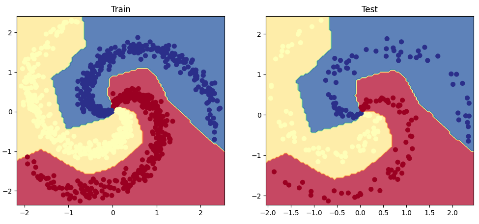
Evaluation
在测试集上评估这个模型。
1
2
3
4
5
6
7
8
9
10
11
12
13
14
15
16
17
18
19
20
21
22
23
24
25
26
27
28
29
30
31
32
33
34
35
36
37
38
39
40
41
42
43
44
45
46
47
48
49
50
51
52
53
54
55
56
57
58
59
60
61
62
63
64
65
66
67
68
69
70
71
72
73
74
75
76
77
78
79
80
81
82
83
84
85
86
87
class MLPFromScratch (): def predict (self, x ): z1 = np.dot(x, W1) + b1 a1 = np.maximum(0 , z1) logits = np.dot(a1, W2) + b2 exp_logits = np.exp(logits) y_hat = exp_logits / np.sum (exp_logits, axis=1 , keepdims=True ) return y_hat model = MLPFromScratch() y_prob = model.predict(X_test) y_pred = np.argmax(y_prob, axis=1 ) performance = get_metrics(y_true=y_test, y_pred=y_pred, classes=classes) print (json.dumps(performance, indent=2 ))def plot_multiclass_decision_boundary_numpy (model, X, y, savefig_fp=None ): """Plot the multiclass decision boundary for a model that accepts 2D inputs. Credit: https://cs231n.github.io/neural-networks-case-study/ Arguments: model {function} -- trained model with function model.predict(x_in). X {numpy.ndarray} -- 2D inputs with shape (N, 2). y {numpy.ndarray} -- 1D outputs with shape (N,). """ x_min, x_max = X[:, 0 ].min () - 0.1 , X[:, 0 ].max () + 0.1 y_min, y_max = X[:, 1 ].min () - 0.1 , X[:, 1 ].max () + 0.1 xx, yy = np.meshgrid(np.linspace(x_min, x_max, 101 ), np.linspace(y_min, y_max, 101 )) x_in = np.c_[xx.ravel(), yy.ravel()] y_pred = model.predict(x_in) y_pred = np.argmax(y_pred, axis=1 ).reshape(xx.shape) plt.contourf(xx, yy, y_pred, cmap=plt.cm.Spectral, alpha=0.8 ) plt.scatter(X[:, 0 ], X[:, 1 ], c=y, s=40 , cmap=plt.cm.RdYlBu) plt.xlim(xx.min (), xx.max ()) plt.ylim(yy.min (), yy.max ()) if savefig_fp: plt.savefig(savefig_fp, format ="png" ) plt.figure(figsize=(12 ,5 )) plt.subplot(1 , 2 , 1 ) plt.title("Train" ) plot_multiclass_decision_boundary_numpy(model=model, X=X_train, y=y_train) plt.subplot(1 , 2 , 2 ) plt.title("Test" ) plot_multiclass_decision_boundary_numpy(model=model, X=X_test, y=y_test) plt.show()
Ending
神经网络是机器学习和人工智能领域的基础,我们必须彻底掌握。
Citation
1
2
3
4
5
6
@article {madewithml, author = {Goku Mohandas} , title = { Neural networks - Made With ML } , howpublished = {\url{https://madewithml.com/} }, year = {2022} }