TL;DR
接上篇,本文使用PyTorch实现一个相同的神经网络模型。
Model
我们将使用两个线性连接层,并在前向传播中添加ReLU激活函数。
1
2
3
4
5
6
7
8
9
10
11
12
13
14
15
16
17
18
19
20
class MLP (nn.Module): def __init__ (self, input_dim, hidden_dim, num_classes ): super (MLP, self).__init__() self.fc1 = nn.Linear(input_dim, hidden_dim) self.fc2 = nn.Linear(hidden_dim, num_classes) def forward (self, x_in ): z = F.relu(self.fc1(x_in)) z = self.fc2(z) return z model = MLP(input_dim=INPUT_DIM, hidden_dim=HIDDEN_DIM, num_classes=NUM_CLASSES) print (model.named_parameters)
Training
训练模型的代码跟之前学到的逻辑回归几乎没有区别。
1
2
3
4
5
6
7
8
9
10
11
12
13
14
15
16
17
18
19
20
21
22
23
24
25
26
27
28
29
30
31
32
33
34
35
36
37
38
39
40
41
42
43
44
45
46
47
48
49
50
51
52
53
54
55
56
57
58
59
LEARNING_RATE = 1e-2 NUM_EPOCHS = 10 BATCH_SIZE = 32 class_weights_tensor = torch.Tensor(list (class_weights.values())) loss_fn = nn.CrossEntropyLoss(weight=class_weights_tensor) def accuracy_fn (y_pred, y_true ): n_correct = torch.eq(y_pred, y_true).sum ().item() accuarcy = (n_correct / len (y_pred)) * 100 return accuarcy optimizer = Adam(model.parameters(), lr=LEARNING_RATE) X_train = torch.Tensor(X_train) y_train = torch.LongTensor(y_train) X_val = torch.Tensor(X_val) y_val = torch.LongTensor(y_val) X_test = torch.Tensor(X_test) y_test = torch.LongTensor(y_test) for epoch in range (NUM_EPOCHS * 10 ): y_pred = model(X_train) loss = loss_fn(y_pred, y_train) optimizer.zero_grad() loss.backward() optimizer.step() if epoch % 10 == 0 : predictions = y_pred.max (dim=1 )[1 ] accuracy = accuracy_fn(y_pred=predictions, y_true=y_train) print (f"Epoch: {epoch} | loss: {loss:.2 f} , accuracy: {accuracy:.1 f} " )
Evaluation
1 2 3 4 5 6 7 8 9 10 11 12 13 14 15 16 17 18 19 20 21 22 23 24 25 26 27 28 29 30 31 32 33 34 35 36 37 38 39 40 41 42 43 44 45 46 47 y_prob = F.softmax(model(X_test), dim=1 ) y_pred = y_prob.max (dim=1 )[1 ] performance = get_metrics(y_true=y_test, y_pred=y_pred, classes=classes) print (json.dumps(performance, indent=2 ))plt.figure(figsize=(12 ,5 )) plt.subplot(1 , 2 , 1 ) plt.title("Train" ) plot_multiclass_decision_boundary(model=model, X=X_train, y=y_train) plt.subplot(1 , 2 , 2 ) plt.title("Test" ) plot_multiclass_decision_boundary(model=model, X=X_test, y=y_test) plt.show()
如你所见,PyTorch的直观和易用性能让我的学习曲线相对平缓。
需要我们编写的核心代码,只集中在定义模型、定义损失函数和优化器、定义训练循环、验证和测试这个四个部分。
当然,还有许多细节需要考虑,比如说数据预处理、模型的保存和加载、使用GPU等。
Initializing weights
到目前为止,我们都是使用了一个很小的随机值初始化权重,这其实不是让模型在训练阶段能够收敛的最佳方式。
我们的目标是初始化一个合适的权重,使得我们激活的输出不会消失或者爆炸,因为这两种情况都会阻碍模型收敛。事实上我们可以自定义权重初始化 方法。目前比较常用的是Xavier初始化方法 和He初始化方法 。
事实上PyTorch的Linear类默认使用了kaiming_uniform_初始化方法,相关源代码看这里 ,后续我们会学习到更高级的优化收敛的策略如batch normalization。
1
2
3
4
5
6
7
8
9
10
11
12
13
14
15
from torch.nn import initclass MLP (nn.Module): def __init__ (self, input_dim, hidden_dim, num_classes ): super (MLP, self).__init__() self.fc1 = nn.Linear(input_dim, hidden_dim) self.fc2 = nn.Linear(hidden_dim, num_classes) def init_weights (self ): init.xavier_normal_(self.fc1.weight, gain=init.calculate_gain("relu" )) def forward (self, x_in ): z = F.relu(self.fc1(x_in)) z = self.fc2(z) return z
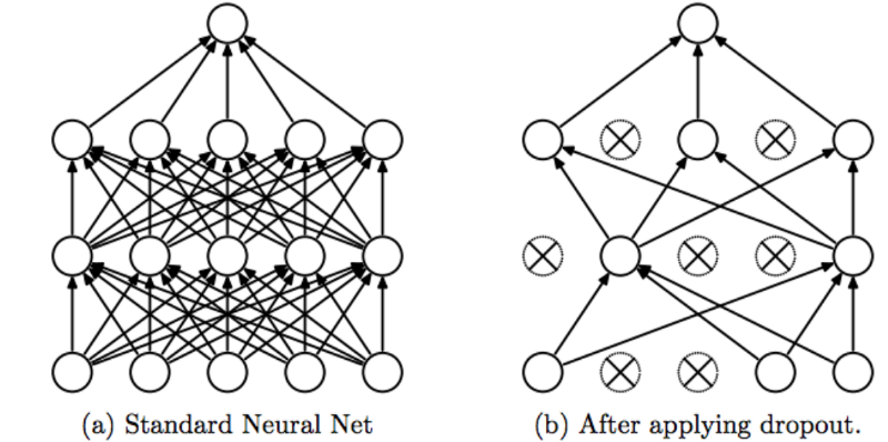
Dropout
能够让我们的模型表现的好的最好的技术是增加数据,但这并不总是一个可选项。幸运的是,还有有一些帮助模型更健壮的其他办法,如正则化、dropout等。
Dropout是在训练过程中允许我们将神经元的输出置0的技术。由于我们每批次都会丢弃一组不同的神经元,所以Dropout可以作为一种采样策略,防止过拟合。
1
2
3
4
5
6
7
8
9
10
11
12
13
14
15
16
17
18
19
20
21
22
23
24
25
26
27
28
29
DROPOUT_P = 0.1 class MLP (nn.Module): def __init__ (self, input_dim, hidden_dim, dropout_p, num_classes ): super (MLP, self).__init__() self.fc1 = nn.Linear(input_dim, hidden_dim) self.dropout = nn.Dropout(dropout_p) self.fc2 = nn.Linear(hidden_dim, num_classes) def init_weights (self ): init.xavier_normal(self.fc1.weight, gain=init.calculate_gain("relu" )) def forward (self, x_in ): z = F.relu(self.fc1(x_in)) z = self.dropout(z) z = self.fc2(z) return z model = MLP(input_dim=INPUT_DIM, hidden_dim=HIDDEN_DIM, dropout_p=DROPOUT_P, num_classes=NUM_CLASSES) print (model.named_parameters)
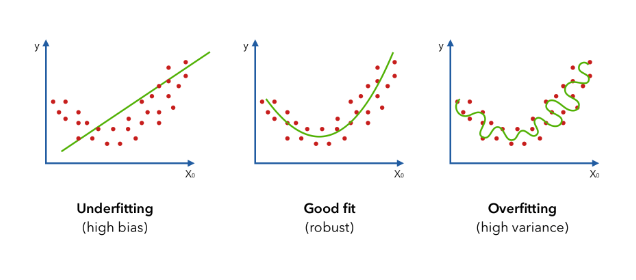
Overfitting
虽然神经网络很擅长捕捉非线性关系,但它们非常容易对训练数据进行过度拟合,且无法对测试数据进行归纳。
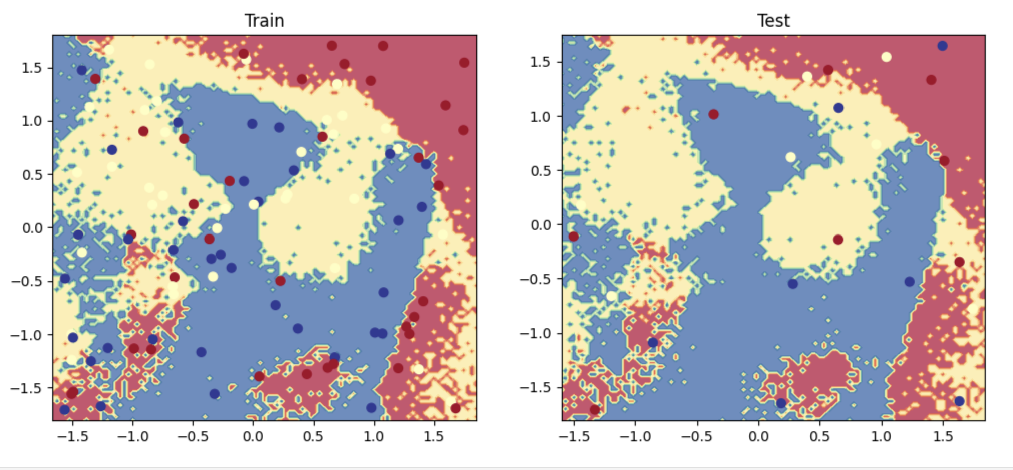
看看下面的例子,我们使用完全随机的数据,并试图拟合含 $2 * N * C + D $ (其中N=样本数,C=标签,D表示输入纬度) 隐藏神经元的模型。
1
2
3
4
5
6
7
8
9
10
11
12
13
14
15
16
17
18
19
20
21
22
23
24
25
26
27
28
29
30
31
32
33
34
35
36
37
38
39
40
41
42
43
44
45
46
47
48
49
50
51
52
53
54
55
56
57
58
59
60
61
62
63
64
65
66
67
68
69
70
71
72
73
74
75
76
77
78
79
80
81
82
83
84
85
86
87
88
89
90
91
92
93
94
95
96
97
98
99
100
101
102
103
104
105
106
107
108
109
110
111
112
113
114
115
116
117
118
119
120
121
122
123
124
125
126
127
128
129
130
131
132
133
134
135
136
137
138
139
140
141
142
143
144
145
146
147
148
149
150
151
152
153
154
155
156
NUM_EPOCHS = 500 NUM_SAMPLES_PER_CLASS = 50 LEARNING_RATE = 1e-1 HIDDEN_DIM = 2 * NUM_SAMPLES_PER_CLASS * NUM_CLASSES + INPUT_DIM X = np.random.rand(NUM_SAMPLES_PER_CLASS * NUM_CLASSES, INPUT_DIM) y = np.array([[i] * NUM_SAMPLES_PER_CLASS for i in range (NUM_CLASSES)]).reshape(-1 ) print ("X: " , format (np.shape(X)))print ("y: " , format (np.shape(y)))X_train, X_val, X_test, y_train, y_val, y_test = train_val_test_split( X=X, y=y, train_size=TRAIN_SIZE) print (f"X_train: {X_train.shape} , y_train: {y_train.shape} " )print (f"X_val: {X_val.shape} , y_val: {y_val.shape} " )print (f"X_test: {X_test.shape} , y_test: {y_test.shape} " )print (f"Sample point: {X_train[0 ]} → {y_train[0 ]} " )X_scaler = StandardScaler().fit(X_train) X_train = X_scaler.transform(X_train) X_val = X_scaler.transform(X_val) X_test = X_scaler.transform(X_test) X_train = torch.Tensor(X_train) y_train = torch.LongTensor(y_train) X_val = torch.Tensor(X_val) y_val = torch.LongTensor(y_val) X_test = torch.Tensor(X_test) y_test = torch.LongTensor(y_test) model = MLP(input_dim=INPUT_DIM, hidden_dim=HIDDEN_DIM, dropout_p=DROPOUT_P, num_classes=NUM_CLASSES) print (model.named_parameters)optimizer = Adam(model.parameters(), lr=LEARNING_RATE) for epoch in range (NUM_EPOCHS): y_pred = model(X_train) loss = loss_fn(y_pred, y_train) optimizer.zero_grad() loss.backward() optimizer.step() if epoch%50 ==0 : predictions = y_pred.max (dim=1 )[1 ] accuracy = accuracy_fn(y_pred=predictions, y_true=y_train) print (f"Epoch: {epoch} | loss: {loss:.2 f} , accuracy: {accuracy:.1 f} " ) y_prob = F.softmax(model(X_test), dim=1 ) y_pred = y_prob.max (dim=1 )[1 ] performance = get_metrics(y_true=y_test, y_pred=y_pred, classes=classes) print (json.dumps(performance, indent=2 ))plt.figure(figsize=(12 ,5 )) plt.subplot(1 , 2 , 1 ) plt.title("Train" ) plot_multiclass_decision_boundary(model=model, X=X_train, y=y_train) plt.subplot(1 , 2 , 2 ) plt.title("Test" ) plot_multiclass_decision_boundary(model=model, X=X_test, y=y_test) plt.show()
正如你所见,虽然模型在训练集上做到了接近70%的准确率,但模型在测试集上的表现并不能令人满意。
重要的是我们需要进行实验,从不合适(高偏差)的简单模型开始,并试图改进到良好的拟合,以及避免过拟合。
Citation
1
2
3
4
5
6
@article {madewithml, author = {Goku Mohandas} , title = { Neural networks - Made With ML } , howpublished = {\url{https://madewithml.com/} }, year = {2022} }