TL;DR

Way2AI系列,确保出发去"改变世界"之前,我们已经打下了一个坚实的基础。

接上篇,本文使用PyTorch实现一个简单的逻辑回归。

Get ready

复用前篇的数据准备及预处理工作,这里直接建模。

Model

我们使用PyTorch的Linear layers 来构建与前篇相同的模型。

1
2
3
4
5
6
7
8
9
10
11
12
13
14
15
16
17
18
19
20
21
22
23
import torch
from torch import nn
import torch.nn.functional as F


class LogisticRegression(nn.Module):
def __init__(self, input_dim, num_classes):
super(LogisticRegression, self).__init__()
self.fc1 = nn.Linear(input_dim, num_classes)

def forward(self, x_in):
z = self.fc1(x_in)
return z


# Initialize model
model = LogisticRegression(input_dim=INPUT_DIM, num_classes=NUM_CLASSES)
print (model.named_parameters)

# Output
# <bound method Module.named_parameters of LogisticRegression(
# (fc1): Linear(in_features=2, out_features=2, bias=True)
# )>

Loss

这里使用交叉熵损失

1
2
3
4
5
6
7
8
9
10
loss_fn = nn.CrossEntropyLoss()
y_pred = torch.randn(3, NUM_CLASSES, requires_grad=False)
y_true = torch.empty(3, dtype=torch.long).random_(NUM_CLASSES)
print (y_true)
loss = loss_fn(y_pred, y_true)
print(f"Loss: {loss.numpy()}")

# Output
# tensor([0, 1, 1])
# Loss: 1.0754622220993042

在这个任务中,我们将数据的类别权重纳入到损失函数中,以对抗样本的类别不平衡。

1
2
3
# Define Loss
class_weights_tensor = torch.Tensor(list(class_weights.values()))
loss_fn = nn.CrossEntropyLoss(weight=class_weights_tensor)

Metrics

我们将在训练模型时引入准确度来衡量模型的性能,因为仅查看损失值并不是非常直观。

后面的章节会介绍相关指标。

1
2
3
4
5
6
7
8
9
10
11
12
# Accuracy
def accuracy_fn(y_pred, y_true):
n_correct = torch.eq(y_pred, y_true).sum().item()
accuracy = (n_correct / len(y_pred)) * 100
return accuracy

y_pred = torch.Tensor([0, 0, 1])
y_true = torch.Tensor([1, 1, 1])
print("Accuracy: {accuracy_fn(y_pred, y_true):.1f}")

# Output
# Accuracy: {accuracy_fn(y_pred, y_true):.1f}

Optimizer

与之前介绍的线性回归一样,这里同样使用Adam优化器。

1
2
3
4
5
from torch.optim import Adam

# Optimizer
LEARNING_RATE = 1e-1
optimizer = Adam(model.parameters(), lr=LEARNING_RATE)

Training

1
2
3
4
5
6
7
8
9
10
11
12
13
14
15
16
17
18
19
20
21
22
23
24
25
26
27
28
29
30
31
32
33
34
35
36
37
# Convert data to tensors
X_train = torch.Tensor(X_train)
y_train = torch.LongTensor(y_train)
X_val = torch.Tensor(X_val)
y_val = torch.LongTensor(y_val)
X_test = torch.Tensor(X_test)
y_test = torch.LongTensor(y_test)

# Training
NUM_EPOCHS = 50
for epoch in range(NUM_EPOCHS):
# Forward pass
y_pred = model(X_train)

# Loss
loss = loss_fn(y_pred, y_train)

# Zero all gradients
optimizer.zero_grad()

# Backward pass
loss.backward()

# Update weights
optimizer.step()

if epoch%10==0:
predictions = y_pred.max(dim=1)[1] # class
accuracy = accuracy_fn(y_pred=predictions, y_true=y_train)
print (f"Epoch: {epoch} | loss: {loss:.2f}, accuracy: {accuracy:.1f}")

# Output
# Epoch: 0 | loss: 0.71, accuracy: 49.6
# Epoch: 10 | loss: 0.23, accuracy: 93.1
# Epoch: 20 | loss: 0.14, accuracy: 97.4
# Epoch: 30 | loss: 0.11, accuracy: 98.3
# Epoch: 40 | loss: 0.09, accuracy: 98.0

Evaluation

首先,我们看看一下测试集的准确率

1
2
3
4
5
6
7
8
9
10
11
12
13
14
15
16
17
18
19
20
21
22
from sklearn.metrics import accuracy_score

# Predictions
pred_train = F.softmax(model(X_train), dim=1)
pred_test = F.softmax(model(X_test), dim=1)
print (f"sample probability: {pred_test[0]}")
pred_train = pred_train.max(dim=1)[1]
pred_test = pred_test.max(dim=1)[1]
print (f"sample class: {pred_test[0]}")

# Output
# sample probability: tensor([0.9934, 0.0066], grad_fn=<SelectBackward0>)
# sample class: 0


# Accuracy (could've also used our own accuracy function)
train_acc = accuracy_score(y_train, pred_train)
test_acc = accuracy_score(y_test, pred_test)
print (f"train acc: {train_acc:.2f}, test acc: {test_acc:.2f}")

# Output
# train acc: 0.98, test acc: 0.97

我们还可以根据其他有意义的指标来评估我们的模型,如精确度和召回率。
$$
accuracy = \frac{TP + FN}{TP + TN + FP + FN}
$$
$$
recall = \frac{TP}{TP + FN}
$$
$$
precision = \frac{TP}{TP + FP}
$$
$$
F1 = 2 * \frac{precision * recall}{precision + recall}
$$

参数 解释
TP truly predicted to be positive and were positive
TN truly predicted to negative and where negative
FP falsely predicted to be positive but where negative
FN falsely predicted to be negative but where positive

格式化指标,以供前端展示

1
2
3
4
5
6
7
8
9
10
11
12
13
14
15
16
17
18
19
20
21
22
23
24
25
26
27
28
29
30
31
32
33
34
35
36
37
38
39
40
41
42
43
44
45
46
47
48
49
50
51
52
53
54
55
import json
import matplotlib.pyplot as plt
from sklearn.metrics import precision_recall_fscore_support

def get_metrics(y_true, y_pred, classes):
"""Per-class performance metrics."""
# Performance
performance = {"overall": {}, "class": {}}

# Overall performance
metrics = precision_recall_fscore_support(y_true, y_pred, average="weighted")
performance["overall"]["precision"] = metrics[0]
performance["overall"]["recall"] = metrics[1]
performance["overall"]["f1"] = metrics[2]
performance["overall"]["num_samples"] = np.float64(len(y_true))

# Per-class performance
metrics = precision_recall_fscore_support(y_true, y_pred, average=None)
for i in range(len(classes)):
performance["class"][classes[i]] = {
"precision": metrics[0][i],
"recall": metrics[1][i],
"f1": metrics[2][i],
"num_samples": np.float64(metrics[3][i]),
}

return performance

# # Performance
performance = get_metrics(y_true=y_test, y_pred=pred_test, classes=label_encoder.classes)
print (json.dumps(performance, indent=2))

# Output
# {
# "overall": {
# "precision": 0.9744444444444446,
# "recall": 0.9733333333333334,
# "f1": 0.9731408308004051,
# "num_samples": 150.0
# },
# "class": {
# "benign": {
# "precision": 1.0,
# "recall": 0.9310344827586207,
# "f1": 0.9642857142857143,
# "num_samples": 58.0
# },
# "malignant": {
# "precision": 0.9583333333333334,
# "recall": 1.0,
# "f1": 0.9787234042553191,
# "num_samples": 92.0
# }
# }
# }

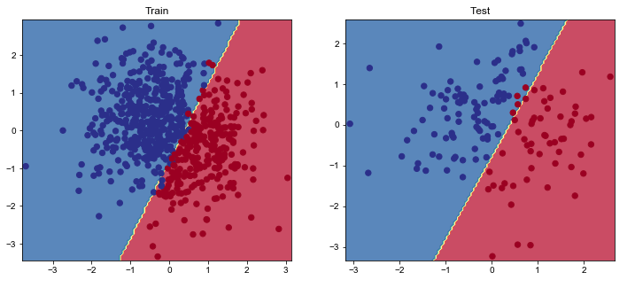
同样的,利用PyTorch实现的逻辑回归模型建模了一个线性决策边界,我们可视化一下结果。

1
2
3
4
5
6
7
8
9
10
11
12
13
14
15
16
17
18
19
20
21
22
23
24
def plot_multiclass_decision_boundary(model, X, y):
x_min, x_max = X[:, 0].min() - 0.1, X[:, 0].max() + 0.1
y_min, y_max = X[:, 1].min() - 0.1, X[:, 1].max() + 0.1
xx, yy = np.meshgrid(np.linspace(x_min, x_max, 101), np.linspace(y_min, y_max, 101))
cmap = plt.cm.Spectral

X_test = torch.from_numpy(np.c_[xx.ravel(), yy.ravel()]).float()
y_pred = F.softmax(model(X_test), dim=1)
_, y_pred = y_pred.max(dim=1)
y_pred = y_pred.reshape(xx.shape)
plt.contourf(xx, yy, y_pred, cmap=plt.cm.Spectral, alpha=0.8)
plt.scatter(X[:, 0], X[:, 1], c=y, s=40, cmap=plt.cm.RdYlBu)
plt.xlim(xx.min(), xx.max())
plt.ylim(yy.min(), yy.max())

# Visualize the decision boundary
plt.figure(figsize=(12,5))
plt.subplot(1, 2, 1)
plt.title("Train")
plot_multiclass_decision_boundary(model=model, X=X_train, y=y_train)
plt.subplot(1, 2, 2)
plt.title("Test")
plot_multiclass_decision_boundary(model=model, X=X_test, y=y_test)
plt.show()

Inference

1
2
3
4
5
6
7
8
9
10
11
12
13
14
15
16
17
18
19
# Inputs for inference
X_infer = pd.DataFrame([{"leukocyte_count": 13, "blood_pressure": 12}])

# Standardize
X_infer = X_scaler.transform(X_infer)
print (X_infer)

# Output
# [[-0.66859939 -3.09473005]]


# Predict
y_infer = F.softmax(model(torch.Tensor(X_infer)), dim=1)
prob, _class = y_infer.max(dim=1)
label = label_encoder.decode(_class.detach().numpy())[0]
print (f"The probability that you have a {label} tumor is {prob.detach().numpy()[0]*100.0:.0f}%")

# Output
# The probability that you have a benign tumor is 90%

Unscaled weights

同样的,我们亦可以逆标准化我们的权重和偏差。

注意到只有$X$被标准化过
$$
\hat{y}_{unscaled} = \sum_{j=1}^k W_{scaled(j)} x_{scaled(j)} + b_{scaled}
$$

已知
$$
\hat{x}_{scaled} = \frac{x_{j} - \overline{x}_{j}}{\sigma_{j}}
$$

于是
$$
\hat{y}_{unscaled} = (b_{scaled} - \sum_{j=1}^k W_{scaled(j)} \frac{\overline{x}_j}{\sigma_{j}}) + \sum_j{\frac{W_{scaled(j)}}{\sigma_j}}x_j
$$

对比公式

$$
\hat{y}_{unscaled} = W_{unscaled} x + b_{unscaled}
$$

便可得知
$$
W_{unscaled} = \frac{W_{scaled(j)}}{\sigma_j}
$$

$$
b_{unscaled} = b_{scaled} - \sum_{j=1}^k W_{unscaled(j)} \overline{x}_j
$$

1
2
3
4
5
6
7
8
9
10
11
12
13
# Unstandardize weights
W = model.fc1.weight.data.numpy()
b = model.fc1.bias.data.numpy()
W_unscaled = W / X_scaler.scale_
b_unscaled = b - np.sum((W_unscaled * X_scaler.mean_))
print (W_unscaled)
print (b_unscaled)

# Output
# [[ 0.80800055 -1.47212977]
# [-0.88854214 0.77129243]]
# [11.4279 13.336911]

Ending

到这里,我们便完成了PyTorch的逻辑回归任务的介绍。

Citation

1
2
3
4
5
6
@article{madewithml,
author = {Goku Mohandas},
title = { Logistic regression - Made With ML },
howpublished = {\url{https://madewithml.com/}},
year = {2022}
}