TL;DR
Way2AI系列,确保出发去"改变世界"之前,我们已经打下了一个坚实的基础。
本文的目标是使用NumPy实现一个多项式逻辑回归模型 $\hat{y}$ ,以实现对给定的特征$X$预测其目标类别的概率分布。
$$
逻辑回归与前篇所述的线性回归,同属于广义线性回归。皆是建模一条直线(或一个平面)。但不同的是,逻辑回归是一种分类模型。
Set up
1
2
3
4
5
6
7
8
import numpy as npimport randomSEED = 1024 np.random.seed(SEED) random.seed(SEED)
Load data
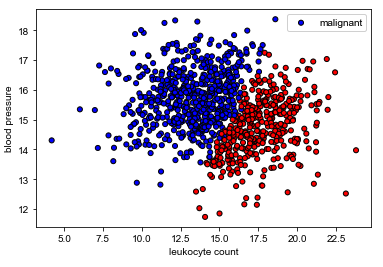
我们的任务是基于白细胞计数和血压来确定肿瘤是否为良性(无害)或恶性(有害)。
请注意,这是一个合成数据集,没有临床意义。
1
2
3
4
5
6
7
8
9
import matplotlib.pyplot as pltimport pandas as pdfrom pandas.plotting import scatter_matrixurl = "http://s3.mindex.xyz/datasets/tumors.csv" df = pd.read_csv(url, header=0 ) df = df.sample(frac=1 ).reset_index(drop=True ) df.head()
1 2 3 4 5 6 7 8 9 10 11 12 X = df[["leukocyte_count" , "blood_pressure" ]].values y = df["tumor_class" ].values colors = {"benign" : "red" , "malignant" : "blue" } plt.scatter(X[:, 0 ], X[:, 1 ], c=[colors[_y] for _y in y], s=25 , edgecolors="k" ) plt.xlabel("leukocyte count" ) plt.ylabel("blood pressure" ) plt.legend(["malignant" , "benign" ], loc="upper right" ) plt.show()
Split data
我们希望将数据集分成三份,使得每个子集中的类别分布相同,以便进行适当的训练和评估。
scikit-learn 提供的方法 train_test_split 可以很容易的做到。
1
2
3
4
5
6
7
8
9
10
11
12
13
14
15
16
17
18
19
20
21
22
23
24
25
26
import collectionsfrom sklearn.model_selection import train_test_splitTRAIN_SIZE = 0.7 VAL_SIZE = 0.15 TEST_SIZE = 0.15 def train_val_test_split (X, y, train_size ): """Split dataset into data splits.""" X_train, X_, y_train, y_ = train_test_split(X, y, train_size=TRAIN_SIZE, stratify=y) X_val, X_test, y_val, y_test = train_test_split(X_, y_, train_size=0.5 , stratify=y_) return X_train, X_val, X_test, y_train, y_val, y_test X_train, X_val, X_test, y_train, y_val, y_test = train_val_test_split( X=X, y=y, train_size=TRAIN_SIZE) print (f"X_train: {X_train.shape} , y_train: {y_train.shape} " )print (f"X_val: {X_val.shape} , y_val: {y_val.shape} " )print (f"X_test: {X_test.shape} , y_test: {y_test.shape} " )print (f"Sample point: {X_train[0 ]} → {y_train[0 ]} " )
现在让我们看一下分割后的数据集中样本分布:
1 2 3 4 5 6 7 8 9 10 11 12 13 14 15 16 17 18 19 20 21 22 class_counts = dict (collections.Counter(y)) print (f"Classes: {class_counts} " )print (f'm:b = {class_counts["malignant" ]/class_counts["benign" ]:.2 f} ' )train_class_counts = dict (collections.Counter(y_train)) val_class_counts = dict (collections.Counter(y_val)) test_class_counts = dict (collections.Counter(y_test)) print (f'train m:b = {train_class_counts["malignant" ]/train_class_counts["benign" ]:.2 f} ' )print (f'val m:b = {val_class_counts["malignant" ]/val_class_counts["benign" ]:.2 f} ' )print (f'test m:b = {test_class_counts["malignant" ]/test_class_counts["benign" ]:.2 f} ' )
可以看出,分割后的数据集里样本分布大体是接近的
Label encoding
注意到我们的分类标签是文本。我们需要将其进行编码,以便在模型中使用。
通常我们使用scikit-learn的LabelEncoder 快速编码。
不过这里我们将编写自己的编码器,以便了解其具体的实现机制。
1
2
3
4
5
6
7
8
9
10
11
12
13
14
15
16
17
18
19
20
21
22
23
24
25
26
27
28
29
30
31
32
33
34
35
36
37
38
39
40
41
42
43
44
45
46
47
48
49
50
51
52
53
54
55
56
57
58
59
60
61
62
63
64
65
66
67
68
69
import itertoolsclass LabelEncoder (object ): """Label encoder for tag labels.""" def __init__ (self, class_to_index={} ): self.class_to_index = class_to_index or {} self.index_to_class = {v: k for k, v in self.class_to_index.items()} self.classes = list (self.class_to_index.keys()) def __len__ (self ): return len (self.class_to_index) def __str__ (self ): return f"<LabelEncoder(num_classes={len (self)} )>" def fit (self, y ): classes = np.unique(y) for i, class_ in enumerate (classes): self.class_to_index[class_] = i self.index_to_class = {v: k for k, v in self.class_to_index.items()} self.classes = list (self.class_to_index.keys()) return self def encode (self, y ): encoded = np.zeros((len (y)), dtype=int ) for i, item in enumerate (y): encoded[i] = self.class_to_index[item] return encoded def decode (self, y ): classes = [] for i, item in enumerate (y): classes.append(self.index_to_class[item]) return classes def save (self, fp ): with open (fp, "w" ) as fp: contents = {'class_to_index' : self.class_to_index} json.dump(contents, fp, indent=4 , sort_keys=False ) @classmethod def load (cls, fp ): with open (fp, "r" ) as fp: kwargs = json.load(fp=fp) return cls(**kwargs) label_encoder = LabelEncoder() label_encoder.fit(y_train) print (label_encoder.class_to_index)print (f"y_train[0]: {y_train[0 ]} " )y_train = label_encoder.encode(y_train) y_val = label_encoder.encode(y_val) y_test = label_encoder.encode(y_test) print (f"y_train[0]: {y_train[0 ]} " )print (f"decoded: {label_encoder.decode([y_train[0 ]])} " )
我们还想计算出类别的权重,这对于在训练期间加权损失函数非常有用。它会告诉模型需要关注样本量不足的类别。
1 2 3 4 5 6 7 8 counts = np.bincount(y_train) class_weights = {i: 1.0 /count for i, count in enumerate (counts)} print (f"counts: {counts} \nweights: {class_weights} " )
Standardize data
我们需要对数据进行标准化处理(零均值和单位方差),以便某个特定特征的大小不会影响模型学习其权重。
这里我们只需要标准化输入$X$,因为我们的输出$y$是离散标签,无须标准化。
1
2
3
4
5
6
7
8
9
10
11
12
13
14
15
16
17
from sklearn.preprocessing import StandardScalerX_scaler = StandardScaler().fit(X_train) X_train = X_scaler.transform(X_train) X_val = X_scaler.transform(X_val) X_test = X_scaler.transform(X_test) print (f"X_test[0]: mean: {np.mean(X_test[:, 0 ], axis=0 ):.1 f} , std: {np.std(X_test[:, 0 ], axis=0 ):.1 f} " )print (f"X_test[1]: mean: {np.mean(X_test[:, 1 ], axis=0 ):.1 f} , std: {np.std(X_test[:, 1 ], axis=0 ):.1 f} " )
Weights
我们的目标是学习一个逻辑回归模型 $\hat{y}$,用来建模自变量 $X$ 与 因变量 $y$ 的关系。
$$
尽管我们的示例任务只涉及两个类别,但我们仍将使用多项式逻辑回归,因为softmax分类器可以推广到任意数量的类别。
第一步 : 随机初始化模型的权重 $W$
1
2
3
4
5
6
7
8
9
10
11
12
INPUT_DIM = X_train.shape[1 ] NUM_CLASSES = len (label_encoder.classes) W = 0.01 * np.random.randn(INPUT_DIM, NUM_CLASSES) b = np.zeros((1 , NUM_CLASSES)) print (f"W: {W.shape} " )print (f"b: {b.shape} " )
Model
第二步 计算输入 $X$ 的对数值($ z = WX $)。然后执行softmax操作得到预测类别的独热编码形式。
举个例子,如果有三个类别,那么一种可能的预测概率是[0.3, 0.3, 0.4]。
1 2 3 4 5 6 7 8 9 10 11 12 13 14 15 16 17 18 19 logits = np.dot(X_train, W) + b print (f"logits: {logits.shape} " )print (f"sample: {logits[0 ]} " )exp_logits = np.exp(logits) y_hat = exp_logits / np.sum (exp_logits, axis=1 , keepdims=True ) print (f"y_hat: {y_hat.shape} " )print (f"sample: {y_hat[0 ]} " )
Loss
第三步 使用代价函数比较预测值 $\hat{y}$ (比如:[0.3, 0.3, 0.4])和目标值 $y$ (比如:[0. 0. 1])来确定损失 $J$。
逻辑回归的常见目标函数是交叉熵损失.
$$
交叉熵损失函数的目标仍然是最小化预测与实际标签之间的差距,从而让模型能够更准确地进行分类.
1 2 3 4 5 6 7 correct_class_logprobs = -np.log(y_hat[range (len (y_hat)), y_train]) loss = np.sum (correct_class_logprobs) / len (y_train) print (f"loss: {loss:.2 f} " )
Gradients
第四步 计算损失函数 $J(\theta)$ 相对于权重的梯度。这里假设我们的类别是互斥的。
$$
1 2 3 4 5 6 y_hat[range (len (y_hat)), y_train] -= 1 y_hat /= len (y_train) dW = np.dot(X_train.T, y_hat) db = np.sum (y_hat, axis=0 , keepdims=True )
Update weights
第五步 指定一个学习率来更新权重 $W$,惩罚错误的分类奖励正确的分类。
1
2
3
4
5
LEARNING_RATE = 1e-1 W == -LEARNING_RATE * dW b += -LEARNING_RATE * db
Training
第六步 : 重复步骤 2 ~ 5,以最小化损失为目的来训练模型
1 2 3 4 5 6 7 8 9 10 11 12 13 14 15 16 17 18 19 20 21 22 23 24 25 26 27 28 29 30 31 32 33 34 35 36 37 38 39 40 41 42 43 44 W = 0.01 * np.random.randn(INPUT_DIM, NUM_CLASSES) b = np.zeros((1 , NUM_CLASSES)) NUM_EPOCHS = 50 LEARNING_RATE = 1e-1 for epoch_num in range (NUM_EPOCHS): logits = np.dot(X_train, W) + b exp_logits = np.exp(logits) y_hat = exp_logits / np.sum (exp_logits, axis=1 , keepdims=True ) correct_class_logprobs = -np.log(y_hat[range (len (y_hat)), y_train]) loss = np.sum (correct_class_logprobs) / len (y_train) if epoch_num%10 == 0 : y_pred = np.argmax(logits, axis=1 ) accuracy = np.mean(np.equal(y_train, y_pred)) print (f"Epoch: {epoch_num} , loss: {loss:.3 f} , accuracy: {accuracy:.3 f} " ) y_hat[range (len (y_hat)), y_train] -= 1 y_hat /= len (y_train) dW = np.dot(X_train.T, y_hat) db = np.sum (y_hat, axis=0 , keepdims=True ) W += -LEARNING_RATE * dW b += -LEARNING_RATE * db
Evaluation
在测试集上评估我们训练好的模型。
1
2
3
4
5
6
7
8
9
10
11
12
13
14
15
16
17
18
19
20
21
22
23
class LogisticRegressionFromScratch (): def predict (self, x ): logits = np.dot(x, W) + b exp_logits = np.exp(logits) y_hat = exp_logits / np.sum (exp_logits, axis=1 , keepdims=True ) return y_hat model = LogisticRegressionFromScratch() logits_train = model.predict(X_train) pred_train = np.argmax(logits_train, axis=1 ) logits_test = model.predict(X_test) pred_test = np.argmax(logits_test, axis=1 ) train_acc = np.mean(np.equal(y_train, pred_train)) test_acc = np.mean(np.equal(y_test, pred_test)) print (f"train acc: {train_acc:.2 f} , test acc: {test_acc:.2 f} " )
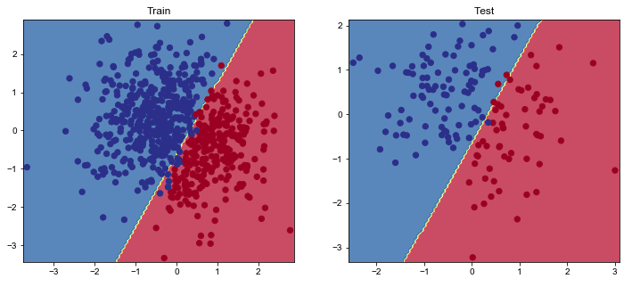
可视化我们的结果
1
2
3
4
5
6
7
8
9
10
11
12
13
14
15
16
17
18
19
20
21
22
23
24
25
26
27
28
29
30
31
32
33
34
35
36
37
38
39
40
def plot_multiclass_decision_boundary (model, X, y, savefig_fp=None ): """Plot the multiclass decision boundary for a model that accepts 2D inputs. Credit: https://cs231n.github.io/neural-networks-case-study/ Arguments: model {function} -- trained model with function model.predict(x_in). X {numpy.ndarray} -- 2D inputs with shape (N, 2). y {numpy.ndarray} -- 1D outputs with shape (N,). """ x_min, x_max = X[:, 0 ].min () - 0.1 , X[:, 0 ].max () + 0.1 y_min, y_max = X[:, 1 ].min () - 0.1 , X[:, 1 ].max () + 0.1 xx, yy = np.meshgrid(np.linspace(x_min, x_max, 101 ), np.linspace(y_min, y_max, 101 )) x_in = np.c_[xx.ravel(), yy.ravel()] y_pred = model.predict(x_in) y_pred = np.argmax(y_pred, axis=1 ).reshape(xx.shape) plt.contourf(xx, yy, y_pred, cmap=plt.cm.Spectral, alpha=0.8 ) plt.scatter(X[:, 0 ], X[:, 1 ], c=y, s=40 , cmap=plt.cm.RdYlBu) plt.xlim(xx.min (), xx.max ()) plt.ylim(yy.min (), yy.max ()) if savefig_fp: plt.savefig(savefig_fp, format ="png" ) plt.figure(figsize=(12 ,5 )) plt.subplot(1 , 2 , 1 ) plt.title("Train" ) plot_multiclass_decision_boundary(model=model, X=X_train, y=y_train) plt.subplot(1 , 2 , 2 ) plt.title("Test" ) plot_multiclass_decision_boundary(model=model, X=X_test, y=y_test) plt.show()
Ending
可以看出,使用NumPy实现的代码相对复杂,下一篇我们即将看到PyTorch是如何便捷的实现逻辑回归。
Citation
1
2
3
4
5
6
@article {madewithml, author = {Goku Mohandas} , title = { Logistic regression - Made With ML } , howpublished = {\url{https://madewithml.com/} }, year = {2022} }