TL;DR
Way2AI系列,确保出发去"改变世界"之前,我们已经打下了一个坚实的基础。
接上篇,本文的目标是使用PyTorch实现一个线性回归模型。
Generate data
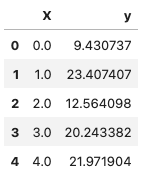
我们复用上篇生成的数据。
1
2
3
4
5
6
7
8
9
10
11
12
13
14
15
16
17
18
19
20
21
22
23
24
25
26
27
28
import numpy as npimport pandas as pdimport matplotlib.pyplot as pltSEED = 1024 NUM_SAMPLES = 50 def generate_data (num_samples ): """Generate dummy data for linear regression.""" X = np.array(range (num_samples)) random_noise = np.random.uniform(-10 , 20 , size=num_samples) y = 3.5 *X + random_noise return X, y X, y = generate_data(num_samples=NUM_SAMPLES) data = np.vstack([X, y]).T df = pd.DataFrame(data, columns=["X" , "y" ]) X = df[["X" ]].values y = df[["y" ]].values df.head()
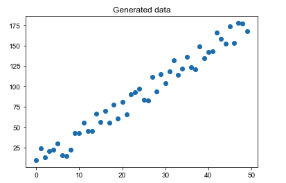
我们将数据绘制成散点图,可以看到它们有很明显的线性趋势。
1 2 3 4 plt.title("Generated data" ) plt.scatter(x=df["X" ], y=df["y" ]) plt.show()
Split data
区别于上一篇中我们使用自定义摇骰子的方式分割数据,这里选择使用scikit-learn 包里提供的train_test_split方法。
1
2
3
4
5
6
7
8
9
10
11
12
13
14
15
16
17
18
19
20
21
22
23
24
25
26
27
28
29
30
from sklearn.model_selection import train_test_splitTRAIN_SIZE = 0.7 VAL_SIZE = 0.15 TEST_SIZE = 0.15 X_train, X_, y_train, y_ = train_test_split(X, y, train_size=TRAIN_SIZE) print (f"train: {len (X_train)} ({(len (X_train) / len (X)):.2 f} )\n" f"remaining: {len (X_)} ({(len (X_) / len (X)):.2 f} )" ) X_val, X_test, y_val, y_test = train_test_split( X_, y_, train_size=0.5 ) print (f"train: {len (X_train)} ({len (X_train)/len (X):.2 f} )\n" f"val: {len (X_val)} ({len (X_val)/len (X):.2 f} )\n" f"test: {len (X_test)} ({len (X_test)/len (X):.2 f} )" )
Standardize data
同样的,我们需要对数据进行标准化处理。这里使用scikit-learn里提供的StandardScaler。
1
2
3
4
5
6
7
8
9
10
11
12
13
14
15
16
17
18
19
20
21
from sklearn.preprocessing import StandardScalerX_scaler = StandardScaler().fit(X_train) y_scaler = StandardScaler().fit(y_train) X_train = X_scaler.transform(X_train) y_train = y_scaler.transform(y_train).ravel().reshape(-1 , 1 ) X_val = X_scaler.transform(X_val) y_val = y_scaler.transform(y_val).ravel().reshape(-1 , 1 ) X_test = X_scaler.transform(X_test) y_test = y_scaler.transform(y_test).ravel().reshape(-1 , 1 ) print (f"mean: {np.mean(X_test, axis=0 )[0 ]:.1 f} , std: {np.std(X_test, axis=0 )[0 ]:.1 f} " )print (f"mean: {np.mean(y_test, axis=0 )[0 ]:.1 f} , std: {np.std(y_test, axis=0 )[0 ]:.1 f} " )
Weights
我们将使用PyTorch的Linear layers来实现一个没有隐含层的神经网络。
1
2
3
4
5
6
7
8
9
10
11
12
13
14
15
16
17
18
19
20
21
22
23
24
25
26
27
28
29
30
31
32
33
34
35
36
37
38
39
40
41
42
43
44
import torchfrom torch import nntorch.manual_seed(SEED) INPUT_DIM = X_train.shape[1 ] OUTPUT_DIM = y_train.shape[1 ] N = 3 x = torch.randn(N, INPUT_DIM) print (x.shape)print (x.numpy())m = nn.Linear(INPUT_DIM, OUTPUT_DIM) print (m)print (f"weights ({m.weight.shape} ): {m.weight[0 ][0 ]} " )print (f"bias ({m.bias.shape} ): {m.bias[0 ]} " )z = m(x) print (z.shape)print (z.detach().numpy())
Model
$$
1
2
3
4
5
6
7
8
9
10
11
12
13
14
15
16
17
18
class LinearRegression (nn.Module): def __init__ (self, input_dim, output_dim ): super (LinearRegression, self).__init__() self.fc1 = nn.Linear(input_dim, output_dim) def forward (self, x_in ): y_pred = self.fc1(x_in) return y_pred model = LinearRegression(input_dim=INPUT_DIM, output_dim=OUTPUT_DIM) print (model.named_parameters)
Loss
同样的,我们使用PyTorch自带的Loss Functions , 这里指定MSELoss.
1
2
3
4
5
6
7
8
loss_fn = nn.MSELoss() y_pred = torch.Tensor([0. , 0. , 1. , 1. ]) y_true = torch.Tensor([1. , 1. , 1. , 0. ]) loss = loss_fn(y_pred, y_true) print ("Loss: " , loss.numpy())
Optimizer
上一篇中我们介绍了使用梯度下降的方法来更新我们的权重。PyTorch中有很多不同的权重更新方法,需要根据不同的场景来选择合适的。详见TORCH.OPTIM 。ADAM optimizer。
1
2
3
4
5
6
from torch.optim import AdamLEARNING_RATE = 1e-1 optimizer = Adam(model.parameters(), lr=LEARNING_RATE)
Training
1 2 3 4 5 6 7 8 9 10 11 12 13 14 15 16 17 18 19 20 21 22 23 24 25 26 27 28 29 30 31 32 33 34 35 36 X_train = torch.Tensor(X_train) y_train = torch.Tensor(y_train) X_val = torch.Tensor(X_val) y_val = torch.Tensor(y_val) X_test = torch.Tensor(X_test) y_test = torch.Tensor(y_test) NUM_EPOCHS = 100 for epoch in range (NUM_EPOCHS): y_pred = model(X_train) loss = loss_fn(y_pred, y_train) optimizer.zero_grad() loss.backward() optimizer.step() if epoch%20 ==0 : print (f"Epoch: {epoch} | loss: {loss:.2 f} " )
Evaluation
现在我们准备评估我们训练好的模型。
1 2 3 4 5 6 7 8 9 10 11 12 13 pred_train = model(X_train) pred_test = model(X_test) train_error = loss_fn(pred_train, y_train) test_error = loss_fn(pred_test, y_test) print (f"train_error: {train_error:.2 f} " )print (f"test_error: {test_error:.2 f} " )
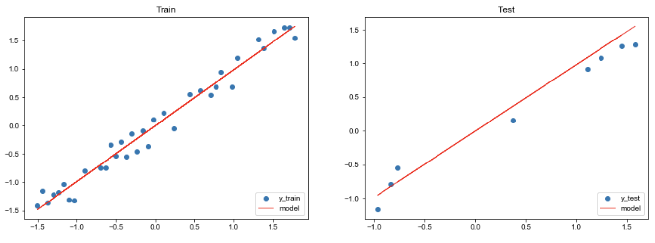
由于我们只有一个特征,因此可以轻松地对模型进行可视化。
1 2 3 4 5 6 7 8 9 10 11 12 13 14 15 16 17 18 19 plt.figure(figsize=(15 ,5 )) plt.subplot(1 , 2 , 1 ) plt.title("Train" ) plt.scatter(X_train, y_train, label="y_train" ) plt.plot(X_train, pred_train.detach().numpy(), color="red" , linewidth=1 , linestyle="-" , label="model" ) plt.legend(loc="lower right" ) plt.subplot(1 , 2 , 2 ) plt.title("Test" ) plt.scatter(X_test, y_test, label='y_test' ) plt.plot(X_test, pred_test.detach().numpy(), color="red" , linewidth=1 , linestyle="-" , label="model" ) plt.legend(loc="lower right" ) plt.show()
Inference
训练完模型后,我们可以使用它来对新数据进行预测。
1 2 3 4 sample_indices = [10 , 15 , 25 ] X_infer = np.array(sample_indices, dtype=np.float32) X_infer = torch.Tensor(X_scaler.transform(X_infer.reshape(-1 , 1 )))
由于我们对数据都进行了标准化,所以对预测值需要进行逆操作。
$$
1 2 3 4 5 6 7 8 9 10 pred_infer = model(X_infer).detach().numpy() * np.sqrt(y_scaler.var_) + y_scaler.mean_ for i, index in enumerate (sample_indices): print (f"{df.iloc[index]['y' ]:.2 f} (actual) → {pred_infer[i][0 ]:.2 f} (predicted)" )
Interpretability
线性回归具有高度可解释性的巨大优势。
1 2 3 4 5 6 7 8 9 10 11 W = model.fc1.weight.data.numpy()[0 ][0 ] b = model.fc1.bias.data.numpy()[0 ] W_unscaled = W * (y_scaler.scale_/X_scaler.scale_) b_unscaled = b * y_scaler.scale_ + y_scaler.mean_ - np.sum (W_unscaled*X_scaler.mean_) print ("[actual] y = 3.5X + noise" )print (f"[model] y_hat = {W_unscaled[0 ]:.1 f} X + {b_unscaled[0 ]:.1 f} " )
Regularization
正则化有助于减少过拟合。本例使用L2正则化 (岭回归)。
通过L2正则化,我们对大的权重值进行惩罚,鼓励权重是较小值。 还有其他类型的正则化,比如L1(套索回归),它可以用于创建稀疏模型,其中一些特征系数被清零,或者结合了L1和L2惩罚的弹性正则化。
正则化不仅适用于线性回归,您可以使用它来处理任何模型的权重,包括我们将在未来学习到的模型。
$$
$$
$$
$\lambda$: 正则化系数; $\alpha$: 学习率
1
2
3
4
5
6
7
8
9
10
11
12
13
14
15
16
17
18
19
20
21
22
23
24
25
26
27
28
29
30
31
32
33
34
L2_LAMBDA = 1e-2 model = LinearRegression(input_dim=INPUT_DIM, output_dim=OUTPUT_DIM) optimizer = Adam(model.parameters(), lr=LEARNING_RATE, weight_decay=L2_LAMBDA) for epoch in range (NUM_EPOCHS): y_pred = model(X_train) loss = loss_fn(y_pred, y_train) optimizer.zero_grad() loss.backward() optimizer.step() if epoch%20 ==0 : print (f"Epoch: {epoch} | loss: {loss:.2 f} " )
1 2 3 4 5 6 7 8 9 10 11 12 13 pred_train = model(X_train) pred_test = model(X_test) train_error = loss_fn(pred_train, y_train) test_error = loss_fn(pred_test, y_test) print (f"train_error: {train_error:.2 f} " )print (f"test_error: {test_error:.2 f} " )train_error: 0.03 test_error: 0.03
对于这个特定的例子,正则化并没有在性能上产生差异,因为我们的数据是从一个完美的线性方程生成的。但是对于大规模真实数据,正则化可以帮助我们的模型很好地泛化。
Ending
本篇基于上一篇的基础,简单介绍了如何用PyTorch实现线性回归。
Peace out.
Citation
1
2
3
4
5
6
@article {madewithml, author = {Goku Mohandas} , title = { Linear regression - Made With ML } , howpublished = {\url{https://madewithml.com/} }, year = {2022} }