TL;DR
Way2AI系列,确保出发去"改变世界"之前,我们已经打下了一个坚实的基础。
本文的目标是使用NumPy实现一个线性回归模型 $\hat{y}$ ,该模型通过最小化预测值和真实值之间的距离来拟合出一条最佳的直线(或一个平面)。
$$
Generate data
我们会生成一些简单的数据,数据大致符合线性分布,但加上一点随机噪声以模拟现实情况( $y = 3.5 * X + 噪声$),意味着这些数据并不完全在一条直线上。
我们的目标是使模型收敛到类似的线性方程上(由于随机噪声的加入,最终的模型结果可能会有差异)。
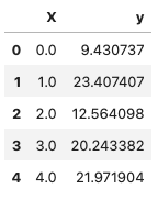
1
2
3
4
5
6
7
8
9
10
11
12
13
14
15
16
17
18
19
20
21
22
23
24
25
26
27
28
import numpy as npimport pandas as pdimport matplotlib.pyplot as pltSEED = 1024 NUM_SAMPLES = 50 def generate_data (num_samples ): """Generate dummy data for linear regression.""" X = np.array(range (num_samples)) random_noise = np.random.uniform(-10 , 20 , size=num_samples) y = 3.5 *X + random_noise return X, y X, y = generate_data(num_samples=NUM_SAMPLES) data = np.vstack([X, y]).T df = pd.DataFrame(data, columns=["X" , "y" ]) X = df[["X" ]].values y = df[["y" ]].values df.head()
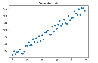
我们将数据绘制成散点图,可以看到它们有很明显的线性趋势。
1 2 3 4 plt.title("Generated data" ) plt.scatter(x=df["X" ], y=df["y" ]) plt.show()
Split data
现在我们已经准备好了数据,接下来需要随机将数据集分成三个部分:训练集、验证集和测试集。
训练集:用来训练我们的模型
验证集:在训练过程中用来检验我们模型的性能
测试集:用来检测我们最终训练好的模型
1
2
3
4
5
6
7
8
9
10
11
12
13
14
15
16
17
18
19
20
21
22
23
24
25
26
27
28
29
30
31
32
33
TRAIN_SIZE = 0.7 VAL_SIZE = 0.15 TEST_SIZE = 0.15 indices = list (range (NUM_SAMPLES)) np.random.shuffle(indices) X = X[indices] y = y[indices] train_start = 0 train_end = int (0.7 *NUM_SAMPLES) val_start = train_end val_end = int ((TRAIN_SIZE+VAL_SIZE)*NUM_SAMPLES) test_start = val_end X_train = X[train_start:train_end] y_train = y[train_start:train_end] X_val = X[val_start:val_end] y_val = y[val_start:val_end] X_test = X[test_start:] y_test = y[test_start:] print (f"X_train: {X_train.shape} , y_train: {y_train.shape} " )print (f"X_val: {X_val.shape} , y_test: {y_val.shape} " )print (f"X_test: {X_test.shape} , y_test: {y_test.shape} " )
Standardize data
我们需要对数据进行标准化处理(零均值和单位方差),这样做的目的是使不同特征之间的值具有可比性,并且能够减少不同特征之间的差异性。
$$
$z$: 标准化后的值; $x_i$: 第i个输入; $\mu$: 平均值; $\sigma$: 标准差
1
2
def standardize_data (data, mean, std ): return (data - mean) / std
需要注意的是,我们将验证集和测试集视为隐藏数据集。因此,我们只使用训练集来确定均值和标准差,以避免偏向我们的训练过程。
1 2 3 4 5 6 7 8 9 10 11 12 13 14 15 16 17 18 19 20 21 22 23 X_mean = np.mean(X_train) X_std = np.std(X_train) y_mean = np.mean(y_train) y_std = np.std(y_train) X_train = standardize_data(X_train, X_mean, X_std) y_train = standardize_data(y_train, y_mean, y_std) X_val = standardize_data(X_val, X_mean, X_std) y_val = standardize_data(y_val, y_mean, y_std) X_test = standardize_data(X_test, X_mean, X_std) y_test = standardize_data(y_test, y_mean, y_std) print (f"mean: {np.mean(X_test, axis=0 )[0 ]:.1 f} , std: {np.std(X_test, axis=0 )[0 ]:.1 f} " )print (f"mean: {np.mean(y_test, axis=0 )[0 ]:.1 f} , std: {np.std(y_test, axis=0 )[0 ]:.1 f} " )
Weights
我们的目标是学习一个模型 $\hat{y}$ ,用权重向量 $W\in\mathbb{R}^{d}$ 和截距 $b\in\mathbb{R}$ 来表达自变量 $X\in\mathbb{R}^{d}$ 与因变量 $y\in\mathbb{R}$ 之间的线性关系:
第一步 : 随机初始化模型的权重 $W$
1
2
3
4
5
6
7
8
9
10
11
12
INPUT_DIM = X_train.shape[1 ] OUTPUT_DIM = y_train.shape[1 ] W = 0.01 * np.random.randn(INPUT_DIM, OUTPUT_DIM) b = np.zeros((1 , 1 )) print (f"W: {W.shape} " )print (f"b: {b.shape} " )
Model
第二步 : 给模型喂 $X$ 以获得预测结果 $\hat{y}$
1 2 3 4 5 6 y_pred = np.dot(X_train, W) + b print (f"y_pred: {y_pred.shape} " )
Loss
第三步 : 通过比较预测值和实际目标值来确定损失 $J$ 。线性回归常见的损失函数是均方误差(MSE)。
1 2 3 4 5 6 7 N = len (y_train) loss = (1 /N) * np.sum ((y_train - y_pred)**2 ) print (f"loss: {loss:.2 f} " )
Gradients
第四步 : 计算损失函数 $J(\theta)$ 的梯度,并更新模型的权重
$$
1 2 3 dW = -(2 /N) * np.sum ((y_train - y_pred) * X_train) db = -(2 /N) * np.sum ((y_train - y_pred) * 1 )
梯度是函数的导数或变化率。它是一个向量,指向函数增长最快的方向。
Update weights
第五步 : 利用一个很小的学习率 $\alpha$ 更新权重
$$
1
2
3
4
5
LEARNING_RATE = 1e-1 W += -LEARNING_RATE * dW b += -LEARNING_RATE * db
Training
第六步 : 重复步骤 2 ~ 5,以最小化损失为目的来训练模型
1
2
3
4
5
6
7
8
9
10
11
12
13
14
15
16
17
18
19
20
21
22
23
24
25
26
27
28
29
30
31
32
33
34
35
36
37
38
NUM_EPOCHS = 100 W = 0.01 * np.random.randn(INPUT_DIM, OUTPUT_DIM) b = np.zeros((1 , )) for epoch_num in range (NUM_EPOCHS): y_pred = np.dot(X_train, W) + b loss = (1 /len (y_train)) * np.sum ((y_train - y_pred)**2 ) if epoch_num%10 == 0 : print (f"Epoch: {epoch_num} , loss: {loss:.3 f} " ) dW = -(2 /N) * np.sum ((y_train - y_pred) * X_train) db = -(2 /N) * np.sum ((y_train - y_pred) * 1 ) W += -LEARNING_RATE * dW b += -LEARNING_RATE * db
为了保持简洁,我们在这里没有计算和显示每个Epoch后的验证集损失。在后续的学习会体现出,在验证集上的表现对训练进程有着至关重要的影响(学习率是否合理、什么时候停止训练等等)
Evaluation
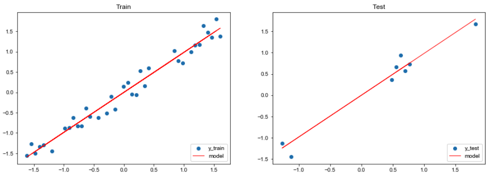
接下来看一下我们训练好的模型在测试数据集上的表现如何。
1 2 3 4 5 6 7 8 9 10 11 pred_train = W*X_train + b pred_test = W*X_test + b train_mse = np.mean((y_train - pred_train) ** 2 ) test_mse = np.mean((y_test - pred_test) ** 2 ) print (f"train_MSE: {train_mse:.2 f} , test_MSE: {test_mse:.2 f} " )
1 2 3 4 5 6 7 8 9 10 11 12 13 14 15 16 17 18 19 plt.figure(figsize=(15 ,5 )) plt.subplot(1 , 2 , 1 ) plt.title("Train" ) plt.scatter(X_train, y_train, label="y_train" ) plt.plot(X_train, pred_train, color="red" , linewidth=1 , linestyle="-" , label="model" ) plt.legend(loc="lower right" ) plt.subplot(1 , 2 , 2 ) plt.title("Test" ) plt.scatter(X_test, y_test, label='y_test' ) plt.plot(X_test, pred_test, color="red" , linewidth=1 , linestyle="-" , label="model" ) plt.legend(loc="lower right" ) plt.show()
Interpretability
由于我们对输入和输出进行了标准化,因此我们的权重适配了这些标准化值。因此,我们需要将权重还原为非标准化状态,以便与真实权重(3.5)进行比较。
$$
已知
$$
于是
进一步可以得到
$$
对比公式
$$
便可得知
$$
1 2 3 4 5 6 7 8 9 W_unscaled = W * (y_std / X_std) b_unscaled = - np.sum (W_unscaled * X_mean) + b * y_std + y_mean print ("[actual] y = 3.5X + noise" )print (f"[model] y_hat = {W_unscaled[0 ][0 ]:.1 f} X + {b_unscaled[0 ]:.1 f} " )
从上面的结果可以看出,我们成功的拟合出了这个线性方程。
Ending
该模型的优势:计算简单,高度可解释, 可以处理连续的和可分类的特征. 而缺点也很明显:只有当数据是线性可分的时候,该模型才能表现良好。
除了回归任务,你也可以将线性回归用于二元分类任务,其中如果预测的连续值高于阈值,则属于某个类别。 不过未来,我们会介绍更好的分类技术。
下一篇,我们将介绍如何用PyTorch实现本篇的内容。
Peace out.
Citation
1
2
3
4
5
6
@article {madewithml, author = {Goku Mohandas} , title = { Linear regression - Made With ML } , howpublished = {\url{https://madewithml.com/} }, year = {2022} }